CSAPP:OptimizationLab #
In this lab we optimize code that evaluates a polynomial and measure its performance ourselves, hoping to deepen understanding of machine-specific optimization and to gain experience measuring performance.
Core materials are taken from our school’s CSAPP lab guide pages.
This also serves as exam review notes.
Preview:
Problems we encounter when optimizing code:
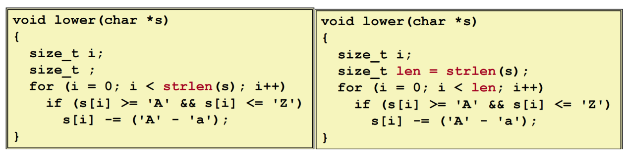
- Function calls — do not call once per loop iteration; try using more temporaries. → code motion
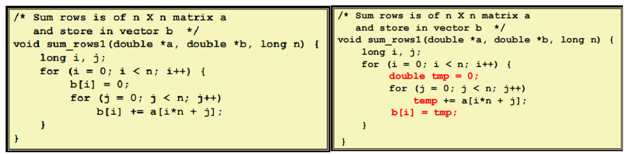
- Memory aliasing — one memory location accessible under two names causes trouble.
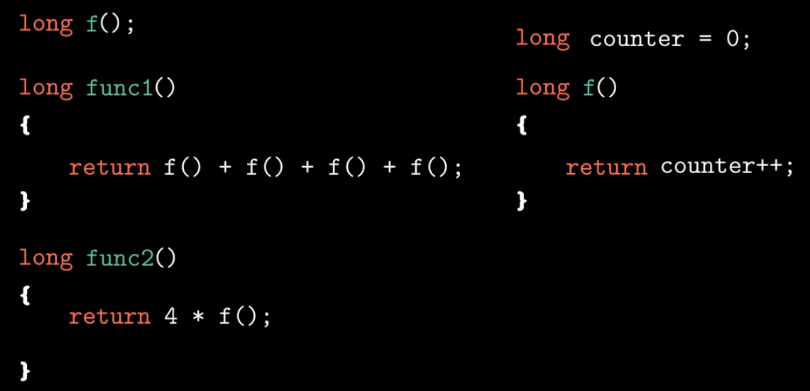
- Repeated function calls — can we just multiply instead?
[!WARNING]
This is actually a common pitfall as well — e.g., issues that arise when iterating with Java’s Iterator. Pay attention to what a function actually does: whether each call has a “persistent” or “cumulative” effect.
Clarify a few concepts first
CPE #
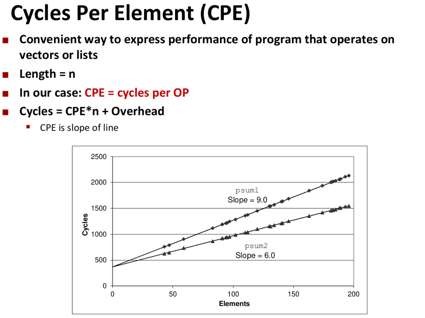
How many clock cycles are needed to process one data element.
For example, in the figure above, a function performs similar work on each element of an array; we can compute how many cycles each element costs — that is CPE.
Treat array length n as the independent variable and cycles consumed as the dependent variable; the slope of the resulting curve is CPE.
Latency Bound #
Latency-bound
As below: when there is a data dependence, computing the next result must wait for the previous computation to finish. That time cannot be reduced — that is the latency bound.
Then the lower bound on CPE is the latency of one floating-point multiply.
double product(double a[], long n)
{
    long i;
    double x = 1.0;
    for (i = 0; i < n; ++i) {
        x *= a[i];
    }
    return x;
}
Throughput Bound #
Throughput-bound
There is no dependence problem; each individual operation is relatively short, but the lower bound comes from having too few execution units available for concurrent work.
Loop Unrolling #
To break through the latency bound toward the throughput bound, eliminate data dependence.
2×1 Unrolling #
Removes some branch prediction cost, but data dependence remains.
for (i = 0; i < limit; i+=2) {
    x = (x OP d[i]) OP d[i+1];
}
2×1a Unrolling #
This shortens the dependence chain.
This is a reassociation transformation.
When OP is addition, it has no effect (in the sense discussed in the notes).
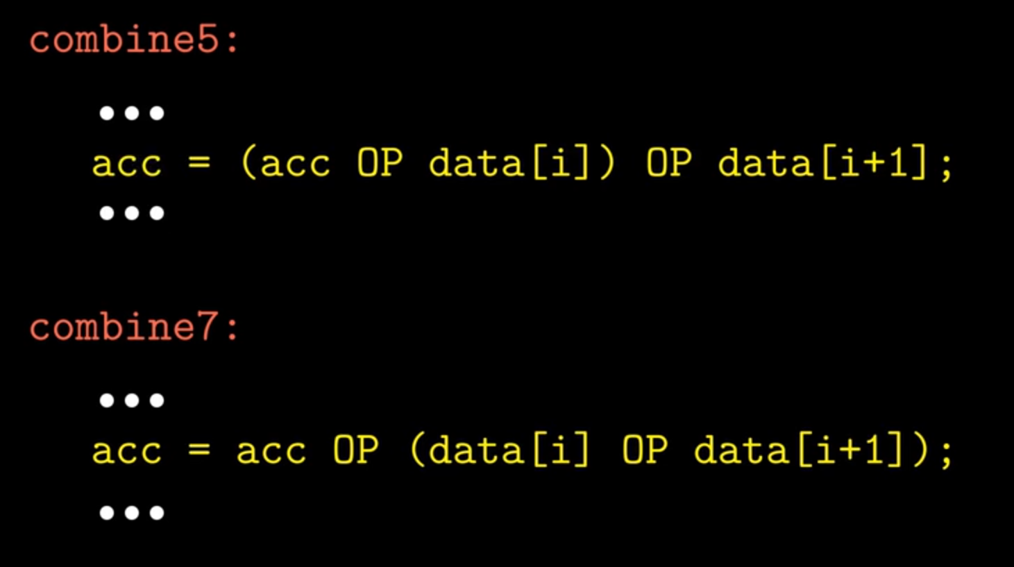
for (i = 0; i < limit; i+=2) {
    x = x OP (d[i] OP d[i+1]);
}
2×2 Unrolling #
Here there are two accumulating product variables, so they can run on two pipelines.
for (i = 0; i < limit; i+=2) {
    x0 = x0 OP d[i];
    x1 = x1 OP d[i+1];
}
K×K Unrolling #
We can unroll aggressively like this, but when there are too many locals, registers run out and memory traffic becomes a new bound.
double product(double a[], long n)
{
    long i;
    double acc1 = 1.0;
    double acc2 = 1.0;
    double acc3 = 1.0;
    double acc4 = 1.0;
    double acc5 = 1.0;
    double acc6 = 1.0;
    double acc7 = 1.0;
    double acc8 = 1.0;
    double acc9 = 1.0;
    double acc10 = 1.0;
    for (i = 0; i + 9 < n; i += 10) {
        acc1 *= a[i];
        acc2 *= a[i + 1];
        acc3 *= a[i + 2];
        acc4 *= a[i + 3];
        acc5 *= a[i + 4];
        acc6 *= a[i + 5];
        acc7 *= a[i + 6];
        acc8 *= a[i + 7];
        acc9 *= a[i + 8];
        acc10 *= a[i + 9];
    }
    acc1 *= acc2;
    acc3 *= acc4;
    acc5 *= acc6;
    acc7 *= acc8;
    acc9 *= acc10;
    acc1 *= acc3;
    acc5 *= acc7;
    for (; i < n; ++i) {
        acc9 *= a[i];
    }
    return acc1 * acc5 * acc9;
}
Part A: Performance Measurement #

void poly(const double a[], double x, long degree, double *result) {
    long i;
    double r = a[degree];
    for (i = degree - 1; i >= 0; i--) {
        r = a[i] + r * x;
    }
    *result = r;
}
This implements Horner’s method to evaluate a polynomial at a point.
I want to measure this function’s CPE.
Many APIs are available; the most recommended is clock_gettime, which can resolve to nanosecond granularity (at least nanosecond units) and can select different clock sources.
Note: when measuring how long this function takes, it is best to run the function once first so the cache already holds the data needed by the call, avoiding large numbers of cache misses that inject unnecessary noise.
The code is simple:
void measure_time(poly_func_t poly, const double a[], double x, long degree,
                  double *time) {
    double result = 0;
    poly(a, x, degree, &result);
    struct timespec start, end;
    clock_gettime(CLOCK_MONOTONIC, &start);
    poly(a, x, degree, &result);
    clock_gettime(CLOCK_MONOTONIC, &end);
    (*time) = end.tv_nsec - start.tv_nsec;
}
Part B: Code Optimization #
For the polynomial algorithm above, what optimizations are available? Roughly loop unrolling and similar techniques — let’s try!
Our goal is to bring this function’s CPE down to 1.
Based on the existing code, we changed the original function to 12×12 loop unrolling.
void poly_optim(const double a[], double x, long degree, double *result) {
 // 此时和秦九公式已经没有关系了,我们想办法最快算出答案即可。
    double acc[12];
    double xpow[13];
    // 记录系数
    acc[0] = a[degree];
    acc[1] = a[degree - 1];
    acc[2] = a[degree - 2];
    acc[3] = a[degree - 3];
    acc[4] = a[degree - 4];
    acc[5] = a[degree - 5];
    acc[6] = a[degree - 6];
    acc[7] = a[degree - 7];
    acc[8] = a[degree - 8];
    acc[9] = a[degree - 9];
    acc[10] = a[degree - 10];
    acc[11] = a[degree - 11];
    // 使用x的哪些幂
    xpow[2] = x * x;
    xpow[3] = xpow[2] * x;
    xpow[4] = xpow[3] * x;
    xpow[5] = xpow[4] * x;
    xpow[6] = xpow[5] * x;
    xpow[7] = xpow[6] * x;
    xpow[8] = xpow[7] * x;
    xpow[9] = xpow[8] * x;
    xpow[10] = xpow[9] * x;
    xpow[11] = xpow[10] * x;
    xpow[12] = xpow[6] * xpow[6];
    // 从倒数12个开始向前进行累积
   int index = degree - 12;
  //  int index = degree - 10;

    while (index >= 11)
    {
        acc[0] = a[index] + acc[0] * xpow[12];
        acc[1] = a[index - 1] + acc[1] * xpow[12];
        acc[2] = a[index - 2] + acc[2] * xpow[12];
        acc[3] = a[index - 3] + acc[3] * xpow[12];
        acc[4] = a[index - 4] + acc[4] * xpow[12];
        acc[5] = a[index - 5] + acc[5] * xpow[12];
        acc[6] = a[index - 6] + acc[6] * xpow[12];
        acc[7] = a[index - 7] + acc[7] * xpow[12];
        acc[8] = a[index - 8] + acc[8] * xpow[12];
        acc[9] = a[index - 9] + acc[9] * xpow[12];
        acc[10] = a[index - 10] + acc[10] * xpow[12];
        acc[11] = a[index - 11] + acc[11] * xpow[12];
        index -= 12;


    }

    // 处理剩下没有计算到的部分
   long remain = (degree + 1) % 12;
    long rest_index = remain;
    double remainValue = 0;
    while (rest_index > 0)
    {
        remainValue *= x;
        remainValue += a[rest_index - 1];
        --rest_index;
    }

    //相当于是一种位移,先把他们之间分开
    double remain1 = acc[0] * xpow[11];
    double remain2 = acc[1] * xpow[10];
    double remain3 = acc[2] * xpow[9];
    double remain4 = acc[3] * xpow[8];
    double remain5 = acc[4] * xpow[7];
    double remain6 = acc[5] * xpow[6];
    double remain7 = acc[6] * xpow[5];
    double remain8 = acc[7] * xpow[4];
    double remain9 = acc[8] * xpow[3];
    double remain10 = acc[9] * xpow[2];
    double remain11 = acc[10] * x + acc[11];
    double mainPart = remain1 + remain2 + remain3 + remain4 + remain5 + remain6 + remain7 + remain8 + remain9 + remain10 + remain11;

    //接着整体向后移位
    index = 0;

    //-----------------------------------------------------------------------------------------------------------
    //
    //	这里我有一个惨痛的教训:
    //	我一开始很长时间把下边循环的限制量写成了rest_index,但是rest_index在上面早就减为0,循环不会再继续
    //	而这里对于答案造成的影响本来就非常非常小,导致我认为是上面的乘法和加法的精度上出了问题,于是浪费了很多时间在更改分块大小观察精度上
    //	直到最后才看到这里出了问题:写的代码再多,有时也会犯这样的错误
    //	1.务必起一个好的变量名,让人知道在干嘛,哪怕是简单的程序
    //	2.想清楚自己在写什么东西,如果是限制量,搞清楚它的大小
    //
    //-----------------------------------------------------------------------------------------------------------
    while(index < remain){
        mainPart *= x;
        ++index;
    }
    (*result) = remainValue + mainPart;
}
Discussion Questions: #
Why does this change bring the function’s CPE to 1? I am only guessing — feel free to leave your thoughts in the comments; honestly I am not fully sure either……
- If
poly()is used to evaluate the polynomial at twoxvalues at once, how does runtime change? What about 14 values? When computing 14 values, is onepoly()that computes them together faster, or callingpoly_optim()14 times?
void poly(const double a[], double x[], long degree, double result[], int n) {
    long i;
    double r[n];
    memset(r, a[degree]);

    for (i = degree - 1; i >= 0; i--) {
        r[0] = a[i] + r[0] * x;
        r[1] = a[i] + r[1] * x;
    }

    for (int index = 0; index < n; ++index){
        result[index] = r[index];
    }
}
Q: Perhaps pass parameters as an array into poly(), with an x array, and still use roughly one loop (roughly as above). Computing two at once should be faster than calling poly twice, but does not remove the dependence. When degree is high, I suspect calling the function 14 times may still be faster.
- Why is the optimized function’s CPE 1 rather than 0.5? Where is the performance bottleneck?
Q: 1. Is -O already the theoretical peak for this function?
Optimized assembly:
	.arch armv8-a
	.file	"poly.c"
	.text
	.align	2
	.global	poly_optim
	.type	poly_optim, %function
poly_optim:
.LFB0:
	.cfi_startproc
	stp	d8, d9, [sp, -64]!
	.cfi_def_cfa_offset 64
	.cfi_offset 72, -64
	.cfi_offset 73, -56
	stp	d10, d11, [sp, 16]
	stp	d12, d13, [sp, 32]
	str	d14, [sp, 48]
	.cfi_offset 74, -48
	.cfi_offset 75, -40
	.cfi_offset 76, -32
	.cfi_offset 77, -24
	.cfi_offset 78, -16
	mov	x5, x0
	ldr	d24, [x0, x1, lsl 3]
	add	x0, x0, x1, lsl 3
	ldr	d23, [x0, -8]
	ldr	d22, [x0, -16]
	ldr	d21, [x0, -24]
	ldr	d20, [x0, -32]
	ldr	d19, [x0, -40]
	ldr	d18, [x0, -48]
	ldr	d17, [x0, -56]
	ldr	d16, [x0, -64]
	ldr	d7, [x0, -72]
	ldr	d6, [x0, -80]
	ldr	d5, [x0, -88]
	ldr	d4, [x0, -96]
	ldr	d3, [x0, -104]
	ldr	d26, [x0, -112]
	fmul	d27, d0, d0
	fmul	d28, d27, d0
	fmul	d29, d28, d0
	fmul	d30, d29, d0
	fmul	d31, d30, d0
	fmul	d8, d31, d0
	fmul	d9, d8, d0
	fmul	d10, d9, d0
	fmul	d11, d10, d0
	fmul	d12, d11, d0
	fmul	d13, d12, d0
	fmul	d14, d13, d0
	fmul	d2, d14, d0
	fmul	d1, d2, d0
	sub	w4, w1, #15
	cmp	w4, 13
	ble	.L2
	add	x3, x5, w4, sxtw 3
.L3:
	fmul	d24, d1, d24
	ldr	d25, [x3]
	fadd	d24, d24, d25
	fmul	d23, d1, d23
	ldr	d25, [x3, -8]
	fadd	d23, d23, d25
	fmul	d22, d1, d22
	ldr	d25, [x3, -16]
	fadd	d22, d22, d25
	fmul	d21, d1, d21
	ldr	d25, [x3, -24]
	fadd	d21, d21, d25
	fmul	d20, d1, d20
	ldr	d25, [x3, -32]
	fadd	d20, d20, d25
	fmul	d19, d1, d19
	ldr	d25, [x3, -40]
	fadd	d19, d19, d25
	fmul	d18, d1, d18
	ldr	d25, [x3, -48]
	fadd	d18, d18, d25
	fmul	d17, d1, d17
	ldr	d25, [x3, -56]
	fadd	d17, d17, d25
	fmul	d16, d1, d16
	ldr	d25, [x3, -64]
	fadd	d16, d16, d25
	fmul	d7, d1, d7
	ldr	d25, [x3, -72]
	fadd	d7, d7, d25
	fmul	d6, d1, d6
	ldr	d25, [x3, -80]
	fadd	d6, d6, d25
	fmul	d5, d1, d5
	ldr	d25, [x3, -88]
	fadd	d5, d5, d25
	fmul	d4, d1, d4
	ldr	d25, [x3, -96]
	fadd	d4, d4, d25
	fmul	d3, d1, d3
	ldr	d25, [x3, -104]
	fadd	d3, d3, d25
	fmul	d26, d1, d26
	ldr	d25, [x3, -112]
	fadd	d26, d26, d25
	sub	w4, w4, #15
	sub	x3, x3, #120
	cmp	w4, 13
	bgt	.L3
.L2:
	add	x3, x1, 1
	mov	x1, -8608480567731124088
	movk	x1, 0x8889, lsl 0
	smulh	x1, x3, x1
	add	x1, x1, x3
	asr	x1, x1, 3
	sub	x0, x1, x3, asr 63
	lsl	x1, x0, 4
	sub	x0, x1, x0
	sub	x0, x3, x0
	cmp	x0, 0
	ble	.L8
	mov	x1, x0
	movi	d25, #0
	sub	x3, x5, #8
.L5:
	fmul	d25, d0, d25
	ldr	d1, [x3, x1, lsl 3]
	fadd	d25, d25, d1
	subs	x1, x1, #1
	bne	.L5
.L4:
	fmul	d1, d2, d24
	fmul	d14, d14, d23
	fadd	d1, d1, d14
	fmul	d13, d13, d22
	fadd	d1, d1, d13
	fmul	d12, d12, d21
	fadd	d1, d1, d12
	fmul	d11, d11, d20
	fadd	d1, d1, d11
	fmul	d10, d10, d19
	fadd	d1, d1, d10
	fmul	d9, d9, d18
	fadd	d1, d1, d9
	fmul	d8, d8, d17
	fadd	d1, d1, d8
	fmul	d31, d31, d16
	fadd	d1, d1, d31
	fmul	d30, d30, d7
	fadd	d1, d1, d30
	fmul	d29, d29, d6
	fadd	d1, d1, d29
	fmul	d28, d28, d5
	fadd	d1, d1, d28
	fmul	d27, d27, d4
	fadd	d1, d1, d27
	fmul	d3, d0, d3
	fadd	d3, d3, d26
	fadd	d1, d1, d3
	cmp	x0, 0
	ble	.L6
	mov	w1, 0
.L7:
	fmul	d1, d1, d0
	add	w1, w1, 1
	cmp	w1, w0
	bne	.L7
.L6:
	fadd	d25, d25, d1
	str	d25, [x2]
	ldp	d10, d11, [sp, 16]
	ldp	d12, d13, [sp, 32]
	ldr	d14, [sp, 48]
	ldp	d8, d9, [sp], 64
	.cfi_remember_state
	.cfi_restore 73
	.cfi_restore 72
	.cfi_restore 78
	.cfi_restore 76
	.cfi_restore 77
	.cfi_restore 74
	.cfi_restore 75
	.cfi_def_cfa_offset 0
	ret
.L8:
	.cfi_restore_state
	movi	d25, #0
	b	.L4
	.cfi_endproc
.LFE0:
	.size	poly_optim, .-poly_optim
	.align	2
	.global	measure_time
	.type	measure_time, %function
Everything is register operations that already avoid memory traffic overhead — and we do not have more multiply units?
Question: what is SIMD-ization?